Selecting sensitive bands from hyperspectral images for plant phenotyping using machine learning algorithms

Ali Moghimi

19 April 2018

Advisors: Ce Yang and Peter Marchetto

Summary

Hyperspectral imaging has recently drawn substantial attention in plant biology field. However, the analysis of hyperspectral images is challenging largely due to the complexity and high-dimensionality of the hyperspectral data. The first objective of this study was to identify predominant spectral features to discriminant pixels representing control and salt treatments. The second objective was to evaluate the feasibility of using the selected spectral features for salt stress phenotyping of four wheat lines. To achieve these goals, we developed an ensemble feature selection pipeline to aggregate the benefits of several feature selection approaches and increase the accuracy of selecting predominant spectral features from hyperspectral images. The ensemble feature selection required solely 15 spectral features out of 215 features to have the minimum classification error of the salt and control pixels. The results showed that we could quantitatively rank the four wheat lines by using only three broad bands centered at: 528, 805, and 589528, 805, and 589 nm.

Significance of feature selection

The importance of feature selection can be viewed from two perspectives:

Data Collection

push-broom hyperspectral camera vs global shutter multispectral camera
cost of hyperspectral camera

Data Analysis

complexity and high-dimensionality of hyperspectral data
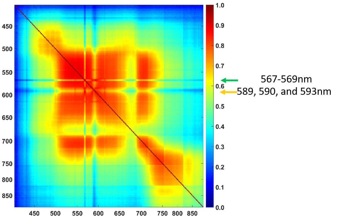
irrelevant and/or redundant features (Figure 1)
risk of overfitting due to large number of redundant features
computational cost and storage
required number of samples (pixels) per each class, ‘the curse of dimensionality’

Objectives

Develop an ensemble feature selection pipeline
- Aggregate the benefits of each feature selection approach
- Identify predominant spectral bands to discriminant pixels representing control and salt treatments.
Generate broad spectral bands from the selected features to develop a low-cost multispectral sensor for salt stress phenotyping
- Evaluate the feasibility of the broad spectral bands to rank four wheat lines based on their tolerance to the imposed salt stress

Methodology

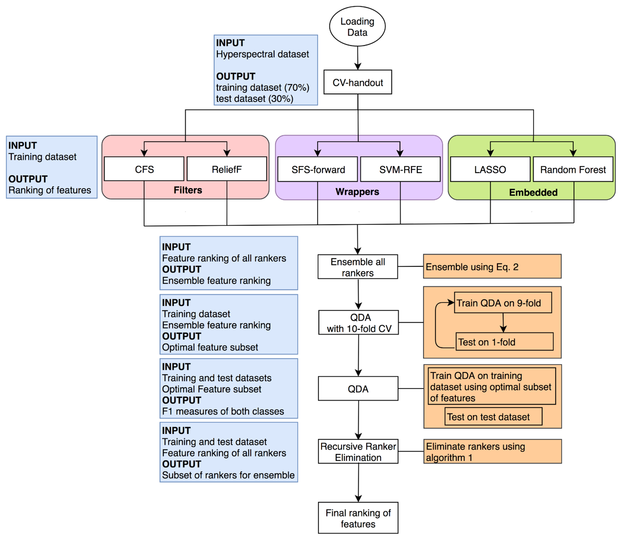
In this study, we used six feature selection rankers as the base rankers of ensemble pipeline, two rankers from each of the three general subsets of feature selection algorithms: filter, wrapper, and embedded methods. Figure 1 shows the flowchart of the proposed ensemble feature selection.

Results

Ensemble of all six rankers results in selecting 18 features to have the highest classification accuracy (77.32%).
Recursive ranker elimination process revealed that the best ensemble is achieved by aggregating only three rankers: ReliefF, SVM-RFE, and Random Forest. This ensemble needed only 15 features to have its highest classification accuracy (77.06%). (Figure 3)
The top-ranked features obtained by the ensemble of three rankers were clustered to form the centers of six multispectral bands: 528, 805, 589, 573, 751, and 546 nm.
Four wheat lines could be ranked based on their tolerance to the imposed salt stress by using these six broad bands. The total ranking error obtained by using these six band compared to using all hyperspectral bands was 1.71%, showing how these six bands could capture most of the spectral information.

Figure 1: High correlation between spectral features. This high correlation indicates the feature redundancy.

Figure 2: Flowchart of the ensemble feature selection to identify predominant spectral features from hyperspectral images.

Figure 3: (a) Ranking of features obtained by the ensemble of reliefF, SVM-RFE, and random forest. (b) The distribution of the 15 selected features over the scanned electromagnetic wavelengths.